Rademacher Complexities
In chapter 4 it has been shown that the property of uniform convergence implies learnability and that the ERM-rule is $\epsilon$-consistent.
In this chapter Rademacher Complexity is introduced which measures the rate of uniform convergence.
Notation:
At first some notation is defined. Given a fixed loss function $\mathcal{l}$ and a hypothesis class $\mathcal{H}$ we define the set of all the projection from a sample $z$ to its loss for the hypothesis class $\mathcal{H}$ as
$\mathcal{F} := \mathcal{l} \circ \mathcal{H} := \{z \mapsto \mathcal{l}(h,z) :h \in \mathcal{H} \} $.
Given some $f \in \mathcal{F} $ define the loss of $f$ over the whole distriburion
$\mathcal{L}_\mathcal{D}(f) := \mathbb{E}_{z \sim \mathcal{D}} [ f(z) ] $
and the loss of $f$ over a sample set $S$ of size $m$ as
$\mathcal{L}_S(f) := \frac{1}{m} \sum _{i=1}^m f(z_i)$.
Finally, define $\mathcal{F} \circ S$ as the set of all possible evaluations a function $f ∈ \mathcal{F}$ can achieve on $S$:
$\mathcal{F} \circ S := \{(f(z_1), \dots,f (z_m)) :f\in \mathcal{F}\}$
Definitions:
The Representativeness of $S$ with respect to $\mathcal{F}$ is defined as
$\text{Rep}_{\mathcal{D}} (\mathcal{F},S) := \sup_{f\in\mathcal{F}} (\mathcal{L}_\mathcal{D} (f) − \mathcal{L}_S (f))$.
It measures the biggest difference of the losses measured over the whole domain and the sample set $S$.
In general it is not possible to calculate the loss of an hypothesis over the whole domain. In practice the representativeness is estimated by splitting up the sample S in some training and validation set.
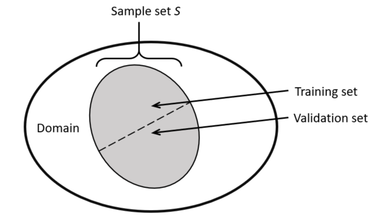
The Rademacher Complexity does exactly this. The sample set $S$ is split up in all possible combinations of training and validation set and the differences in the losses are averaged.
$\mathcal{R}(\mathcal{F} \circ S) := \frac{1}{m} \mathop{\mathbb{E}}_{\sigma \sim \{\pm 1\}^m } [ \sup _{f \in \mathcal{F} } \sum_{i=1}^{m} \sigma_i f ( z_i ) ] $
The definition makes use of $\sigma \sim \{\pm 1\}^m$ assigning a sample $z_i$ either to the training or validation set where $\sigma$ i.i.d. with $\mathbb{P}[ \sigma_i = 1] = \mathbb{P} [ \sigma_i = − 1] = \frac{1}{2} $.
Lemmas and Theorems:
Lemma 26.2 bounds the expected value of representativeness of $S$ by twice the expected Rademacher Complexity.
$ \mathop{\mathbb{E}} _{S \sim \mathcal{D}^m} [ \text{Rep}_\mathcal{D} (F,S )] \leq 2 \mathop{\mathbb{E}} _{S \sim \mathcal{D}^m} \mathcal{R} ( \mathcal{F} \circ S) $
This implies that by splitting up the sample $S$ into different validation and training sets one can actually estimate the (expected value of the) loss difference between sample $S$ and the distribution $\mathcal{D}$.
Lemma 26.2 can be applied directly to the Representativeness of a specific hypothesis, for example $\text{ERM}_\mathcal{H}(S)$ or some $h^*$ (Theorem 26.3).
In general, we want to bound the expected value of the representaticeness of $S$ with a better dependence on the confidence parameter $\delta \in (0,1)$. This is achieved by applying the McDiarmid’s Inequality which leads to Theorem 26.5.
This theorem requires, that for all samples $z$ and all hypotheses $h \in \mathcal{H}$ their loss needs to be bounded by a constant $| \mathcal{l} ( h,z ) | \leq c$. Then,
(i) With probability of at least $1 − \delta$ and for all $h \in \mathcal{H}$
$\mathcal{L}_\mathcal{D} (h) − \mathcal{L}_S (h) \leq 2 \mathop{\mathbb{E}} _{S’ \sim \mathcal{D}^m} [ \mathcal{R} ( \mathcal{l} \circ \mathcal{H} \circ S’ ) ] + c \sqrt{ \frac{2 ln( 2 / \delta)}{m} }$ .
In particular, this holds for $h = \text{ERM}_\mathcal{H} ( S )$ .
(ii) With probability of at least $1 − \delta$ and for all $h \in \mathcal{H}$
$\mathcal{L}_\mathcal{D} (h) − \mathcal{L}_S (h) \leq 2 \mathcal{R} ( \mathcal{l} \circ \mathcal{H} \circ S) + 4 c \sqrt{ \frac{2 ln( 4 / \delta )}{m} } $.
In particular, this holds for $h = \text{ERM}_\mathcal{H} ( S )$.
(iii) For any $h^*$ and with probability of at least $1 − \delta$,
$\mathcal{L}_\mathcal{D} ( \text{ERM}_\mathcal{H} ( S ) ) − \mathcal{L}_\mathcal{D} (h^*) \leq 2 \mathcal{R} ( \mathcal{l} \circ \mathcal{H} \circ S) + 5 c \sqrt{ \frac{2 \ln( 8 / \delta)}{m} } $.
The above theorem 26.5 gives three different bounds that mainly say, that, if the Rademacher Complexity $\mathcal{R}(\mathcal{l} \circ \mathcal{H} \circ S)$ is small, the ERM-rule can be used. Also the second and third bound depend on the chosen sample set $S$, which is called a data-dependent bound and in comparison to other bounds, the third bound can be calculated since it doesn’t involde an expected value over the distribution $\mathcal{D}$!
Rademacher Calculus:
Four Properties where proven for Rademacher Calculus which can be applied to bound the Rademacher Complexity $\mathcal{R}(\mathcal{l} \circ \mathcal{H} \circ S)$ for specific cases.
For a set $A \subset \mathbb{R}^m$
- When applying an affine transformation with factor $c \in \mathbb{R}$ and translation $a_0 \in \mathbb{R}^m$ to $A$, it holds $\mathcal{R}(\{ca + a_0 : a \in A \}) \leq | c | \mathcal{R} (A) $
- The Rademacher Complexity of the complex hull of $A$ is equal to the Rademacher Complexity of $A$
- Massart lemma: The Rademacher Complexity of a finite set grows logarithmically with its size.
- Contraction lemma: If in every dimension $i \in [m]$ of $A$ a $\rho$-Lipschitz function $\varphi_i:\mathbb{R} \to \mathbb{R}$ is applied, the Rademacher complexity of the transformed $\Phi(A)$ can be bounded via $\mathcal{R}(\Phi(A)) \leq \rho \mathcal{R}(A)$.
Rademacher Complexity of Linear Classes:
The following two linear and bounded hypothesis classes will be analyzed in detail applying some of the properties for Rademacher Calculus:
$\mathcal{H}_1 = \{ x \mapsto \langle w , x \rangle : \| w \|_1 \leq 1 \}$
$\mathcal{H}_2 = \{ x \mapsto \langle w , x \rangle : \| w \|_2 \leq 1 \}$
The Rademacher Complexity of the hypothesis class $\mathcal{H}_2$ can be bounded by the maximum $\mathcal{l}_2$-norm of an instance from Hilbert space $S$ devided by the square root of $m$, the size of $S$ (Lemma 26.10).
$\mathcal{R}(\mathcal{H}_2 \circ S ) \leq \max_i \frac{ \|x_i\|_2 }{ \sqrt{m} }$
Notice that the dimension of the Hilbert space $S = \{x_1, \dots, x_m\}$ does not influence the Rademacher complexity $\mathcal{R}(\mathcal{H}_2 \circ S)$, which is usefull when analyzing kernel methods.
A similar bound can be proven for the Rademacher Complexity of $\mathcal{H}_1$, but the dimension of $S \subset \mathbb{R}^n$ does appear in the numerator of the bound (Lemma 26.11).
$\mathcal{R}(\mathcal{H}_1 \circ S ) \leq \max_i \|x_i\|_\infty \frac{ 2 \log(2n) }{ \sqrt{m} }$
Apart from the extra $\log(n)$ factor that appears in Lemma 26.11, a comparison of both bounds is interesting. In Lemma 26.10, $w$ is bounded by its $\mathcal{l}_2$-norm and the $\mathcal{l}_2$-norm of the instances influences the bound. In contrast, in Lemma 26.11 $w$ is bounded by its $\mathcal{l}_1$-norm (which is stronger than an $\mathcal{l}_2$-constraint) while the $\mathcal{l}_\infty$-norm of the instances should be low since it appears in the numerator (which is weaker than a low $\mathcal{l}_2$ assumption).
| Hypothesis Class | Bounds on hypotheses ($w$) | Bounds on instances $x$ |
|---|---|---|
| $\mathcal{H}_1$ | $\mathcal{l}_1$-norm | $\mathcal{l}_\infty$-norm |
| $\mathcal{H}_2$ | $\mathcal{l}_2$-norm | $\mathcal{l}_2$-norm |
Therefore, the choice of the hypothesis class $\mathcal{H}$ and a constraint on instances and hypotheses should depend on our prior knowledge of the set of instances and on prior assumptions on good predictors.
Questions:
Q: On the page 376 in the very first line $\sigma$ is introduced. Should the distribution of -1 and +1 be equal?
A: Yes, since we further assume that the sizes of the two disjoint sets are equal.
Q: Page 378. Formula on the top of the page: would it suffice if $h^*$ is Lipschitz continuous?
A: Yes, but we have to bound something. (for Lipschitz - domain).
Observation: Theorem 26.5 - 3. is a remarkable result: if we learn our S, we have learnt the overall distribution pretty much.
Q: Lemma 26.8 - why do they use maximum of differences between estimated and actual $a$?
A: They use the geometric idea of difference between mean and center, where center is an actual $a$.
Q: Lemma 26.10 - why does not hold for $\mathcal{H}_1$?
A: The $\mathcal{v}$ can be bounded by whatever.
Q: Can we use $\mathcal{l}_1$-norm for kernel methods?
A: No there is dimension under the square root.
Q: Theorem 26.13 bounds probability of misclassification. Why do they use $\mathcal{R}$-value in statement and not in the proof?
A: Value $\mathcal{c}$ which was used previously (for example in Theorem 26.12) in front of the square root is bounded by this $\mathcal{R}$-value.